1 Introduction
In the quest for artificial general intelligence, three main paradigms have been adopted in the field of machine learning to empower a machine, or rather have it learn to perform tasks without giving it specific instructions to do so: Supervised learning, Unsupervised learning, and Reinforcement learning.
Reinforcement learning, which is the main subject of this series of articles, is conceptualized on the idea that a machine (or agent) can learn to do any task if given reward signals by maximizing them. [1].
2 The framework
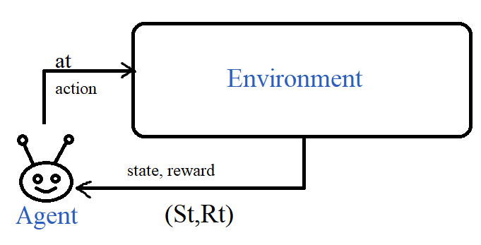
In their simplest form, RL problems are modelled by an agent interacting with an environment at the time step \( t \) by choosing an action \( a_t \) while in state \( S_t \) and the environment returns a reward \( R_t \) and transitions to the next state \( S_{t+1} \).
Whatever the horizon of the problem, the goal of the agent is choosing a policy \( \pi \) to maximize the sum of expected rewards:
\[ \mathbb{E}_{p(a_0, s_1, a_1, \ldots, a_T, s_T \mid s_0, \pi)} \left[ \sum_{t=0}^T R(s_t, a_t) \,\middle|\, s_0 \right] \]
A task can either be continual whereas the agent continues to interact with the model forever, or episodic, where interactions are terminated in a state called terminal state that returns a reward of 0 and updates to itself. Once an episode ends, it is possible to enter a new one where the initial state \( s_0 \) is randomized and the episode or trajectory length \( T \) can be different, when \( T \) is finite, we call the problem a finite horizon problem.
In this case, the return to maximize is the sum of discounted rewards where each reward is multiplied by a discount factor \( \gamma \).
\[ \mathbb{E}_{p(a_0, s_1, a_1, \ldots, a_T, s_T \mid s_0, \pi)} \left[ \sum_{t=0}^{\infty} \gamma^{t} r_t \mid s_0 = s \right] \]
The discount factor is there to ensure that the agent does not act in a myopic manner in which he will always try to maximize the immediate reward by choosing an action he knows has the highest reward without further exploring if there are any other actions with a higher reward.
We make certain assumptions about the environment:
- Memorylessness: \[ p(s_{t+1} \mid s_t, a_t, s_{t-1}, a_{t-1}, \dots, s_0, a_0) = p(s_{t+1} \mid s_t, a_t). \]
- Full observability: The agent is able to observe the full state environment.
Several approaches are used to learn optimal policies mainly: Value-based, Policy-based and Model-Based, in the next chapter we will present Value-based methods.
References
References
- David Silver, Satinder Singh, Doina Precup, Richard S. Sutton, Reward is enough, Artificial Intelligence, Volume 299, 2021, 103535.